Tectogrammatical Parsing

Category Graphs and Head Chains

Tectogrammatical parsing (tecto-parsing) is performed after pheno-parsing. The tecto-parsing algorithm used in ALE is a specialised head-corner parsing algorithm. Head, in the sense that we require here, must only be a lexical category that is sure to be found inside its phrasal category. For example, one is sure to find a verb in all sentences. In general, this can be a syntactic head, a semantic head, or any other obligatory and lexical category which is computationally advantageous to look for first.

Our tectogrammatical parser is based on the one discussed in Penn and Haji-Abdolhosseini (2002,2003), and our tectogrammatical rules are those of the Linear Specification Language (LSL, Goetz and Penn, 1997) extended to incorporate topological fields and splicing; LSL itself has a compaction constraint but does not name the resulting contiguous fields/regions, and defines no phenogrammatical structure. Parsing with parallel phenogrammatical and tectogrammatical structures is also very reminiscent of Ahrenberg's (1989) much earlier proposal to separate linear precedence and contiguity from semantic interpretation in LFG parsing.

Suhre (1999) presented a bottom-up parser for LSL that used an ordered graph to represent the right-hand-sides of rules, and multiple Earley-style ``dots'' in the graph to track the progress of chart edges through their rules. Daniels and Meurers (2002) re-branded LSL as ``Generalised ID/LP'' (GIDLP), and proposed a different Earley-style parser. In their parser, only one ``dot'' is used, and the order in which categories are specified by a grammar-writer (which no longer implicitly states linear precedence assumptions) is used to guide the search for rule daughters. Our parser, although not Earley-style, follows Daniels and Meurers (2002) in using this specification order as a guide. In particular, the heads of a particular category are taken to be those lexical categories accessible by a chain through exclusively leftmost daughters in the specification order. In our view, however, Earley deduction is not sufficiently goal-oriented to be suitable for parsing in a freer word-order language.

We call the chain of head daughters down to a preterminal a head chain. For example, a head chain for S in the grammar fragment presented in Figure 10.6 is VP-V. By static analysis of the grammar, ALE can also calculate minimum and maximum heights for each chain as well as minimum and maximum yields at any given height for each category. Height refers to the number of categories below a given node in a syntactic tree. According to the grammar in Figure 10.6 for example, an N occurs at height 1 because there is a lexical item under it and N' occurs at height 2 because there are two nodes under it, namely N and a lexical item. Yield or more precisely phonological yield refers to the number of words that a given category encompasses. For example in the grammar in Figure 10.6, the yield of an N' can be either 1 (for just a N) or 2 (for a Det and an N). We will discuss this in more detail below.

In order to calculate minimum and maximum heights and yields, given a set of grammar rules, ALE generates a graph for those rules at compile time. There are two types of nodes in each graph: category nodes (depicted as circles), and rule nodes (depicted as squares). Circular nodes are called category nodes because they could be thought of as representing the left-hand-side of a rule in the grammar. Square nodes are called rule nodes because they could be thought of as the categories in the body (right-hand-side) of a rule. In a category graph, category nodes and rule nodes alternate; i.e., a circular node only points to one or more square node(s), and a square node only points to one or more circular node(s). Figure 10.6 shows a small piece of grammar and the graph that ALE generates based on it.

The maximum yield of category $X$ at a maximum height $h$ is:

$$X_{max}(\leq h) = \max_{0\leq j\leq h} X_{max}(j)$$

The minimum yield of category $X$ at a maximum height $h$ is:

$$X_{min}(\leq h) = \min_{0\leq j\leq h} X_{min}(j)$$

These are useful for cases when $X_{max}(h)$ and $X_{min}(h)$ for a given $h$ is not defined. They also provide a convenient notation for defining the equations derived from tecto-rules.

For every category $X$, $X_{max}(h)$ is simply defined as the sum of the maximum yields of its daughters at $h-1$ (or lower). It could be, however, that a smaller height tree for $X$ actually has a bigger yield than $X$ at height exactly $h$ because trees at certain multiples of heights could be formed by disjoint combinations of rules. So in the general case, the formula for $X_{max}(h)$ takes the form:

$$\textrm{S}_{max}(h) = \max\left\{ \begin{array}{l} \textr... ...P}_{max}(\leq h-1)+\textrm{VP}_{max}(h-1) \end{array} \right.$$

This ensures that the tree from which we choose the maximum yield is in fact of height $h$.

We likewise define $X_{min}(h)$ as the sum of the minimum yields of its daughters (which are at height $h-1$). This is defined as the $X_{min}(h-1)$ of one daughter plus the $X_{min}(\leq h-1)$ of other daughters. To decide for which daughter we need to calculate $X_{min}(h-1)$ and for which we need to calculate $X_{min}(\leq h-1)$, we have to calculate all possibilities and then take the smallest number. For instance, S$_{min}(h)$ is calculated as follows:

$$\textrm{S}_{min}(h) = \min\left\{ \begin{array}{l} \textr... ...P}_{min}(\leq h-1)+\textrm{VP}_{min}(h-1) \end{array} \right.$$

Lexical items and empty categories always occur at height 0. Lexical items always have a minimum and maximum yield of 1. Empty categories have a minimum and maximum yield of 0. Lexical categories (preterminals) always occur at height 1 and have minimum and maximum yield of 1. These are the square nodes that directly project from the lexicon. For acyclic rules, calculating $X_{min}$ and $X_{max}$ is very simple because acyclic categories (such as N' in our sample grammar) always have the same minimum and maximum yields and occur at the same height. For example, an N' always occurs at height 2 (lexical items are at height 0, and preterminals are at height 1); and N'$_{min}(2)=1$, N'$_{max}(2)=2$. This is because we have N' $\to$ N and N' $\to$ N Det in this grammar fragment.

Because tecto-rules do not assume order or contiguity, performing bottom-up parsing in the same manner as pheno-parsing is ill-advised. Not using active edges in the parser is also not a very wise approach. Tecto-parsing is performed top-down but in a very goal-oriented fashion in order to prune search. Before an active edge is added to chart, the parser uses head chains in order to make sure that the lexical category that must necessarily be present inside a category really is present. If the parser fails to find the head chain that is required for making the category it is predicting, it will not add the corresponding active edge to the chart. To prune search even further, ALE takes into account the minimum and maximum yields of categories at any given height. If given the number of words and explicit precedence and topological constraints ALE finds out that it can never consume all of the input or it requires more words to build an edge. It will not add that active edge to the chart.

Bit Vector Lattices

As mentioned in the previous section, an active edge contains two bit vectors: CanBV and OptBV. CanBV represents the words that the edge is allowed to take, and OptBV represents the words that it is allowed not to take. At run time, we frequently see that an active edge gets added to the chart that only slightly differs from another active edge that has already been introduced to the chart. For example, let us assume that the chart already includes an active edge with the CanBV 00001111 and the OptBV 11110000, and another edge with the same category and with the CanBV 00001011 and the OptBV 11110100 gets added to the chart. It is obvious that the two edges differ only in one bit (namely the third bit): in the first edge, the bit belongs to the CanBV, but in the second edge, it belongs to the OptBV. In cases like this, when a new active edge differs only slightly with an existing one, we want to make sure that we adjust our search space so that we do not redo the search that we did when the first edge was added to the chart. Table 10.1 shows all the possible basic situations that may arise in such a case. For ease of exposition, we will not use actual bit vectors here and instead use number sets to stand for the word numbers in the input string. For example, {1,2,3} under the CanBV column means that the edge is allowed to take the first, second, and third words from the input string (which is equivalent to the bit vector 000111) in this example. The last column of Table 10.1 shows the subsumption condition that must hold in a unification-based setting. Here A stands for the category of the first edge and B for the category of the second edge.

Table 10.1: Possible relationships between the bit vectors of two similar active edges

		CanBV	OptBV	Subsumption Condition
1.	a.	{1,2,3}	{4,5,6}
	b.	{1,2}	{3,4,5,6}	B $\sqsubseteq$ A
2.	a.	{1,2,3}	{4,5,6}
	b.	{1,2}	{4,5,6}	A $\sqsubseteq$ B
3.	a.	{1,2,3}	{4,5,6}
	b.	{1,2,3,4}	{5,6}	A $\sqsubseteq$ B
4.	a.	{1,2,3}	{4,5,6}
	b.	{1,2,3}	{5,6}	A $\sqsubseteq$ B
5.	a.	{1,2,3}	{4,5,6}
	b.	{1,2,3}	{4,5,6,7}	B $\sqsubseteq$ A
6.	a.	{1,2,3}	{4,5,6}
	b.	{1,2,3,7}	{4,5,6}	A $\sqsubseteq$ B

As is shown in Table 10.1, there are six basic situations. The rows marked `a' represent the bit vectors of the first active edge, and the rows marked `b' represent the bit vectors of the new active edge. In the first situation, a word moves from the CanBV to the OptBV. In the second situation, a word drops from the CanBV. In the third, a word moves from OptBV to CanBV, and in the fourth, a word drops from OptBV. In the fifth and sixth situation, a word is added to OptBV and CanBV respectively.

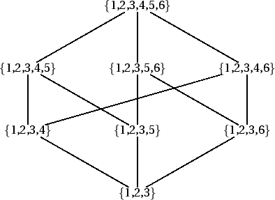
In order to understand the relationships of these situations with respect to the search space that we need to cover, it helps to think of the bit vectors in terms of lattices of word sets. Let the bottom of the lattice stand for the set corresponding to CanBV and the top stand for the set corresponding to CanBV $\vee$ OptBV. In this case, the order relation is defined with set inclusion meaning that $x < y$ iff $x \subset y$. For example, the lattice corresponding to the bit vectors in Table 10.1 item 1a, is shown in Figure 10.7.

Figure 10.7: The lattice representation of the bit vectors in Table 10.1 item 1a

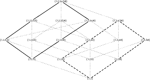
What the lattice in Figure 10.7 means is having an active edge with the CanBV of {1,2,3} and OptBV of {4,5,6} entails having already covered the search spaces provided by CanBV {1,2,3,4}, {1,2,3,5}, etc. and the same OptBV. Let us now see what happens in the first situation given in Table 10.1. If one word moves from CanBV to OptBV, it means that we have given our lattice a new bottom, {1,2}. The new lattice corresponding to the new search space is shown in Figure 10.8.

Figure 10.8: The lattice representation of the bit vectors in Table 10.1 item 1a

The lattice of Figure 10.7 is a sub-lattice of the one in Figure 10.8, which means that the new active edge overlaps in its search space with that of the old one. What the parser does in this case is to adjust the bit vectors to CanBV {1,2} and OptBV {4,5,6} thus restricting the search space to the part of the lattice shown in dashed lines. This means that case 1 in Table 10.1 effectively reduces to case 2.

The third, fourth, and fifth cases are simple. In all these cases, the lattice representation of the new active edge is a sub-lattice of the old one, which means that the search space has already been covered and the parser does not need to do anything. In these cases, the edge will not be added to the chart. It is only in the last case that the parser cannot make use of the existing information and has to perform a full search by adding the edge to the chart intact. This is because the lattice representation of the new edge is completely disjoint from the old one.